Photonic quantum computing,
simulated and compared.
Two kinds of work: schemes from the literature reproduced in our own simulators, and PQCF's photonic kernels measured against five other simulators every week.
PQCF against the photonic simulators,
head to head, every week.
The photonic simulators benchmark each other on four tasks: the permanent, the torontonian, boson-sampling throughput and Fock-space simulation of a 10-mode quantum neural network. The papers show these benchmarks as graphs, each on its own hardware:
- Piquasso: Kolarovszki et al., arXiv:2403.04006, Quantum 9, 1708 (2025), Figs. 7, 10 and 11.
- DeepQuantum: He et al., arXiv:2512.18995, Fig. 3.
Neither includes PQCF. We ran the same four tasks with PQCF and five other programs on the same inputs, the same machine and the same core, with one thread each:
- The Walrus 0.22.0 (JOSS 2019);
- Piquasso 8.0.2;
- Perceval 1.3.1 (arXiv:2204.00602);
- DeepQuantum 4.5.0;
- Strawberry Fields 0.23.0 (arXiv:1804.03159).
Every program's answers are checked against the others'. The suite now runs every week, and each run's tables are published.
The tasks:
- The permanent of an n × n block of a random unitary.
- The torontonian, used in boson sampling with threshold detectors (arXiv:1807.01639), of a strongly squeezed k-mode Gaussian state.
- Exact boson sampling (arXiv:1011.3245): n photons in n² modes. PQCF and Perceval use Clifford and Clifford's algorithm (arXiv:1706.01260).
- One layer of a continuous-variable quantum neural network (arXiv:1806.06871) on 10 modes, in Fock space.
Every answer agrees: 51 of 51 checks in the first run. The number depends on how many sizes each program reaches within the 120-second limit: in the run of 15 November, DeepQuantum needed 123 s for one torontonian, so its next size was not run and that run has 50 checks, all agreeing. Every run now names the sizes it skipped, and a run in which a program gives no results fails as incomplete.
- Permanents and torontonians agree with The Walrus to within 1e-8.
- Every program's boson samples pass a chi-square test against the exact distribution.
- Piquasso's Fock states match PQCF's to 5e-16.
Time, one core (in brackets, the time relative to PQCF's):
| task | PQCF | The Walrus | Piquasso | Perceval | DeepQuantum |
|---|---|---|---|---|---|
| permanent, n = 24 | 0.59 s | 0.47 s (0.8×) | 0.39 s (0.66×) | 0.34 s (0.57×) | 58.6 s (99×) |
| permanent, n = 28 | 11.1 s | 8.6 s (0.78×) | 7.7 s (0.7×) | 6.4 s (0.58×) | — |
| torontonian, k = 20 | 0.40 s | 1.40 s (3.6×) | 0.17 s (0.43×) | — | 25.0 s (63×) |
| torontonian, k = 24 | 8.0 s | 27.1 s (3.4×) | 3.0 s (0.37×) | — | 546 s (68×) |
| boson sampling, exact samples per second | PQCF | Piquasso | Perceval | DeepQuantum |
|---|---|---|---|---|
| 4 photons, 16 modes | 1,324,328 | 4,624 | 19,973 | 33,686 |
| 8 photons, 64 modes | 121,855 | 334 | 1,997 | — (lists every output first) |
| 12 photons, 144 modes | 5,700 | 121 | 199 | — |
| 16 photons, 256 modes | 264 | 36.9 | 19.7 | — |
| 20 photons, 400 modes | 12.8 | 3.16 | — (at most 256 modes) | — |
| Fock simulation, 10 modes | states kept | seconds | truncation error |
|---|---|---|---|
| PQCF, at most 10 photons in total | 184,756 | 1.10 | — |
| Piquasso, the same states | 184,756 | 0.35 | 5e-16 from PQCF |
| PQCF, at most 8 photons in total | 43,758 | 0.23 | 3e-7 |
| DeepQuantum, at most 4 photons per mode | 1,048,576 | 0.15 | 5e-4 |
| Strawberry Fields, at most 4 photons per mode | 1,048,576 | 10.9 | 5e-4 |
What this says about PQCF, plainly:
- Its boson sampler is the fastest at every size: 4 to 360 times faster than Piquasso, and 13 to 66 times faster than Perceval.
- Its permanent is the slowest of the four compiled programs. Perceval is 1.7 times faster and Piquasso 1.4 times.
- Its torontonian is second. Piquasso's recursive algorithm (arXiv:2109.04528) is 2.7 times faster, while PQCF is 3.4 times faster than The Walrus.
- Its Fock backend is 3 times slower than Piquasso's on the same states.
These three gaps are now the targets for PQCF's kernels. DeepQuantum's GPU paths were not compared: this is one CPU core.
Found on the way: Piquasso computes wrong permanents on ARM processors.
- The cause: its C++ stores a sign in a plain
char, which is unsigned on ARM, so −1 becomes 255. - The effect: the permanent of [[1, 2], [3, 4]] comes out as 522 instead of 10.
- In our comparison, Piquasso is built with signed chars, as on x86, and its answers are then exact.
A mistake of ours, also written down. Our first torontonian inputs were weakly squeezed, so the probability that every mode clicks was tiny (1e-13). The torontonian's 2k terms then cancelled, and every program's answer at k = 22 to 24 was numerical noise. The inputs are now squeezed as in Gaussian boson sampling experiments, and the answers agree to 1e-10.
The latest tables, every run, the method and the code: comparison/photonic (latest results).
How to reproduce the results: a step-by-step page: every simulator at a fixed version, one at a time on one core, about 13 minutes; it says how to compare your times with ours. It runs here every Sunday.
Photons on a beamsplitter, the KLM gates,
fusion, detectors and loss.
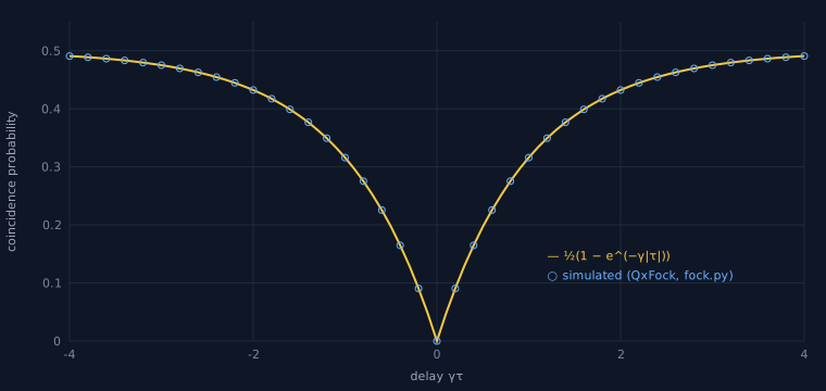
What this is. Simulations of schemes from the literature — not photonic hardware. A photon simulator in Fock space, written twice from one conventions file (docs/optics_conventions.md): QxFock in Elixir (this service) and fock.py in the TechUPGRADE engine. Each applies an interferometer two ways (expanding creation operators; permanents by Ryser's formula). On 60 random interferometers of 4–8 modes and 1–4 photons, every output amplitude agrees: the two routes to 1e-15, Python with Perceval (Quandela) to 2e-16, Elixir with Python to 2 × 10⁻¹⁵; one beamsplitter sign flipped shows as 0.61.
Hong–Ou–Mandel. Two photons meet on a balanced beamsplitter; when they overlap fully they always leave together. With exponential pulses offset by τ (overlap e^(−γ|τ|/2)) the coincidence probability is ½(1 − e^(−γ|τ|)): simulated at 81 delays, it matches to 2e-16 and is exactly 0 at τ = 0.
The KLM gates (Knill, Laflamme, Milburn, Nature 409, 46, 2001). The nonlinear sign gate, from KLM's own 3-mode unitary and from the beamsplitter form (angles 22.5°, 65.5302°, −22.5° and a π phase): on 50 random inputs α₀|0⟩ + α₁|1⟩ + α₂|2⟩ it gives α₀|0⟩ + α₁|1⟩ − α₂|2⟩ with probability 1/4 and fidelity 1 − 10⁻¹⁵. Two of them make a CZ on dual-rail qubits (8 modes, 4 photons): process fidelity 1 − 3 × 10⁻¹⁶, success exactly 1/16.
Checks that bite, and one that did not. The middle angle off by 0.5° lowers the CZ fidelity to 0.9997. Leaving out the π phase was expected to break the gate; it does not — it gives diag(1, −1, −1) per NS gate, and the circuit becomes CZ followed by Z on both qubits, still a CZ up to single-qubit phases. So that is no power check, and we say so.
Fusion (Browne and Rudolph, PRL 95, 010501, 2005). Type-I fusion, simulated photon by photon — polarising beamsplitter, 45° rotation, one polarisation-resolving detector — acts on the two input qubits as (|0⟩⟨00| ± |1⟩⟨11|)/√2 (to 10⁻¹⁶), succeeds with the input's weight on |HH⟩ and |VV⟩ (½ for cluster qubits), and its failures are Z measurements of both. Type II succeeds with probability ½ and projects onto one Bell state, Φ⁺ or Ψ⁺: linear optics tells apart two of the four. On state vectors, fusing the ends of linear clusters of n and m qubits (2–5) gives the cluster of n + m − 1 with fidelity 1 − 2 × 10⁻¹⁶.
Growing a chain. A long linear cluster grows by fusing k-qubit pieces onto its end, each piece itself built from Bell pairs by fusion; on a failure the chain loses its end qubit and the piece its first. Bell pairs used per qubit gained (Monte Carlo, 20 × 20,000 attempts):
| piece, qubits | leftover discarded | leftover reused |
|---|---|---|
| 2 | never | never |
| 3 | 7.98 ± 0.04 | 7.01 ± 0.04 |
| 4 | 9.07 ± 0.04 | 7.01 ± 0.03 |
| 5 | 10.65 ± 0.03 | 7.68 ± 0.02 |
| 6 | 12.48 ± 0.02 | 8.46 ± 0.02 |
Bell pairs alone (k = 2) never grow the chain — success adds one qubit, failure takes one away. Three-qubit pieces cost 8 pairs per qubit, or 7 when the two-qubit leftover of a failure is reused: the review's "2 × 4 − 1 = 7". Its "6.5" we do not find in any strategy we simulated; the best are 7.0, with three- or four-qubit pieces and reuse (data, fusion checks, /quantum/optics/fusion).
Measurement-based computation (on state vectors). One-bit teleportation through a two-node cluster and a rotation along a chain (adaptive angles, Pauli byproducts) reach fidelity 1 on random inputs. The review's four-node example does not hold as drawn: its Fig. 10 chain (CZ₁₂CZ₂₃CZ₃₄) gives a CZ between the teleported input and the fourth qubit — CNOT-class by its local invariants, but needing gates before as well as after; the couplings its Eq. 56 writes (1–2, 2–3, 2–4) do give a CNOT for every outcome and for superposition inputs, with Pauli byproducts when built from CZ gates (data).
Detectors and loss. A detector of efficiency η is a beamsplitter onto an empty mode before an ideal detector: its outcome probabilities match the bucket and number-resolving formulas (the review's Eqs. 80–81) to 4 × 10⁻¹⁶. Through such detectors on the heralds, lost photons make false heralds; with bucket detectors, which cannot tell one photon from two, the gates fail even at η = 1:
| η | NS fidelity, resolving | bucket | CZ fidelity on |++⟩, resolving | bucket | CZ herald rate |
|---|---|---|---|---|---|
| 1.00 | 1.0000 | 0.7216 | 1.0000 | 0.4667 | 0.0625 |
| 0.99 | 0.9941 | 0.7199 | 0.9836 | 0.4639 | 0.0623 |
| 0.95 | 0.9702 | 0.7130 | 0.9210 | 0.4529 | 0.0612 |
| 0.90 | 0.9398 | 0.7045 | 0.8493 | 0.4395 | 0.0596 |
| 0.80 | 0.8796 | 0.6877 | 0.7256 | 0.4139 | 0.0551 |
| 0.50 | 0.7271 | 0.6404 | 0.4714 | 0.3466 | 0.0331 |
And a photon lost from a dual-rail qubit leaves exactly ηρ + (1 − η)|vac⟩⟨vac| (to 2 × 10⁻¹⁶): an erasure, heralded by the missing photon — the error model of our next step, decoding erasures (data, CSV).
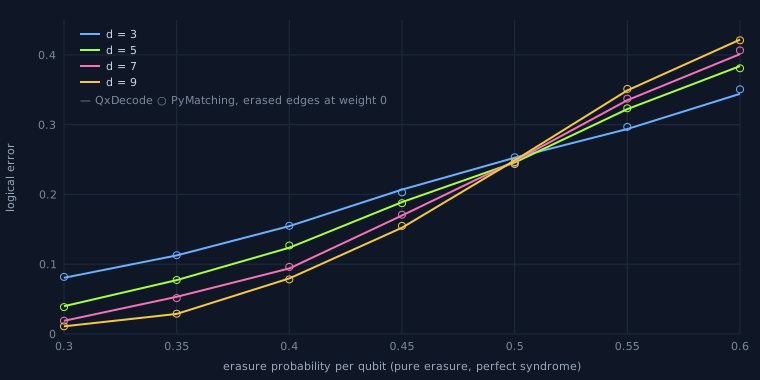
Erasure decoding — the part that is ours. A lost photon is a heralded erasure: the qubit is known to hold a random Pauli. Our union-find decoder, QxDecode, takes erased edges as already grown and weightless in the peeling tree — for pure erasure the peeling decoder of Delfosse and Zémor, which is maximum-likelihood. At code capacity (the rotated surface code, perfect syndrome, 20,000 shots a point, PyMatching with the erased edges at weight 0 on the same shots beside it), pure erasure crosses at 50 % for d = 3 to 9, the percolation threshold, and the two decoders agree:
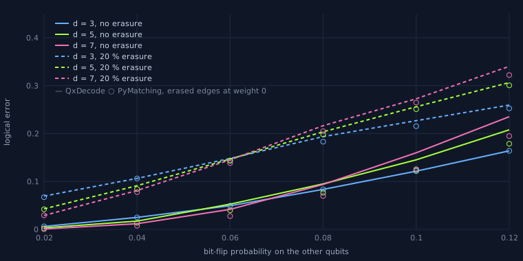
With bit flips on the other qubits the crossing falls as the erased share grows — near 8–10 % of flips without erasure, about 8 % with 10 % erasure, about 6 % with 20 % — in line with the usual linear trade-off; QxDecode is a little less accurate than matching without erasure (as union-find is) and close to it once erasures dominate:
At circuit level, QxStab samples heralded erasure (Stim's HERALDED_ERASE semantics; on a d = 3 memory with 2 % erasure its 51 detectors and 27 heralds agree with Stim's sampler, exact tests, smallest corrected p 0.89). Surface-code memories, d rounds, Pauli noise 0.1 % on every operation and heralded erasure on every data qubit each round; the decoding graph from Stim's error model, each herald mapped to the edges its erasure can flip; 20,000 shots a point:
| d | erasure per round | QxDecode, with heralds | PyMatching, with heralds | PyMatching, ignoring them |
|---|---|---|---|---|
| 3 | 0 % | 0.06 % | 0.05 % | 0.05 % |
| 3 | 2 % | 0.29 % | 0.29 % | 1.31 % |
| 3 | 4 % | 0.66 % | 0.64 % | 2.99 % |
| 3 | 8 % | 1.51 % | 1.49 % | 8.48 % |
| 5 | 0 % | 0.01 % | 0.01 % | 0.01 % |
| 5 | 2 % | 0.03 % | 0.06 % | 0.65 % |
| 5 | 4 % | 0.12 % | 0.10 % | 2.70 % |
| 5 | 8 % | 0.47 % | 0.41 % | 9.96 % |
| 7 | 0 % | 0.00 % | 0.00 % | 0.00 % |
| 7 | 2 % | 0.03 % | 0.03 % | 0.34 % |
| 7 | 4 % | 0.04 % | 0.03 % | 1.82 % |
| 7 | 8 % | 0.14 % | 0.14 % | 10.43 % |
Knowing where the losses were is worth about twenty times in logical error at d = 5 and 4 % erasure, and keeps larger codes better even at 8 % per round — where, without the heralds, the larger code is already worse. QxDecode uses the heralds about as well as matching does (data, pure-erasure data, mixed data, tools/erasure/).
The 2.7 % loss figure. Romero and Milburn's review (p. 27) says fusion-based computation "can tolerate a 2.7 % probability of suffering a single-photon loss". It comes from Bartolucci et al. (Nat. Commun. 14, 912, 2023, Sec. VI and Appendix B): the 6-ring fusion network with (2,2)-Shor-encoded resource states and fusions boosted with a Bell pair (failure 1/4, four photons per fusion). We reproduce it from their formulas — 2.71 % per photon, which is 10.4 % that at least one of the four photons is lost, and their 43.2 % failure threshold at zero loss — taking their simulated erasure threshold (11.98 %) as given; we have not simulated the fusion network itself. Unencoded, the same network tolerates no loss at failure 1/4; the 4-star network, encoded, about 1.0 % (tools/optics/fbqc_loss.py).
One mode: GKP and cat qubits (Gottesman, Kitaev, Preskill, PRA 64, 012310, 2001; Ralph et al., PRA 68, 042319, 2003). A third simulator, for one optical mode in continuous variables, again written twice: cv.py in Python works in the Fock basis and on a grid in q, QxCV in Elixir on the grid alone, its p side summed analytically over the peaks instead of by FFT. Squeezed vacuum from the Fock basis matches the closed-form wavefunction to 8 × 10⁻¹⁵, and Eq. 24 holds to 9 × 10⁻¹⁴. Eq. 26 holds only if the phases of Eqs. 22 and 25 agree: with ζ = re^(−2iϕ) as printed, the rotation must be e^(+iϕ), not Eq. 25's e^(−iϕ) (flipping either sign works); as printed, the variances are off by up to 5.6 when ϕ ≠ 0.
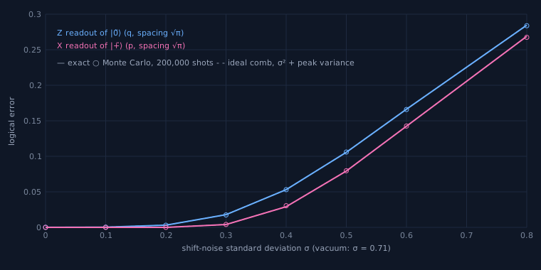
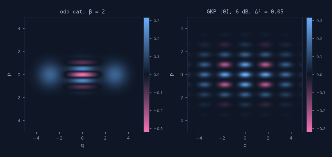
GKP states (Eq. 38; α = √π, peaks squeezed 10 dB, Δ² = 0.01). The logical Z̄ = e^(iπq/α) reads ±0.924 on |0̃⟩ and |1̃⟩, equal to an analytic sum over the Gaussian peaks to 10⁻¹⁰; X̄ = e^(−ipα) takes |0̃⟩ to |1̃⟩ with fidelity 0.984 — the envelope does not move with the peaks — also as predicted. Read out after a Gaussian shift of σ, the logical error from the exact integral, from 200,000 sampled readouts, and from the closed form for an ideal comb with σ² plus the peak's variance agree (the closed form to 1.5 × 10⁻⁷), in q and in p. Eq. 39's bounds show as an error of ½ (to 2 × 10⁻⁵) at a shift of α/2 in q or π/2α in p. QxCV's X readout (the Fourier sum) and Python's (the FFT) agree to 10⁻¹³:
The review's Fig. 5, read from the vector curve in its PDF. The peaks sit at multiples of √π, as Eq. 38 gives with α = √π; each peak's variance fits 0.11 — near e^(−2r) = 0.09 for r = 1.2, while the caption says e^(2r) = 11; and the |1̃⟩ envelope falls off four times faster than the |0̃⟩ one (4.00), which a single Δ in Eq. 38 cannot give. With the caption's Δ̃ = 0.01, amplitudes e^(−Δ̃(sα)²) for |0̃⟩ and e^(−Δ̃[(2s+1)α]²) for |1̃⟩ fit both panels: the |0̃⟩ panel looks drawn with s where Eq. 38 has 2s.

Cat states (Eq. 75). From the Fock basis and from the grid they agree to 10⁻¹⁵; they hold only even or only odd photon numbers, and the Wigner function at the origin is ⟨Π⟩/π = ±1/π (to 2 × 10⁻¹⁶). Eq. 40's N±⁻¹ leaves the state with norm² 1/N±; Eq. 75's N±^(−1/2) is right. Photon loss is the cat code's error — one lost photon flips the parity — and after a loss 1 − η, ⟨Π⟩ = cosh(β²(1 − 2η))/cosh β² for the even cat (sinh for the odd): the generating function (QxCV) and the Fock amplitudes thinned photon by photon (Python) agree to 2 × 10⁻¹⁶.
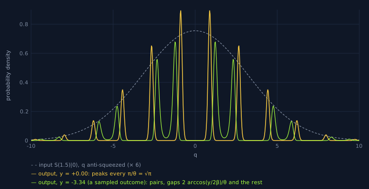
A comb heralded by homodyne detection (Eqs. 66–73). With Eq. 69's Kraus amplitude the outcomes y sum to one for every q (to 10⁻⁹); Eq. 70 as printed sums to 1/√2 — it lacks the ½ in the exponent. A phase-squeezed input with the outcome y = 0 gives peaks every π/θ (√π here: a GKP-like comb); other outcomes give pairs, with gaps 2 arccos(y/2β)/θ and the rest of the period, as sampled:
checks · Elixir against Python · readout · Eq. 39 shifts · Fig. 5 as read · comb · tools/optics/cv_checks.py, xcheck_cv.py · /quantum/optics/gkp, /cat, /comb
From the review we started from (Romero and Milburn, arXiv:2404.03367): its Fig. 8 gives the third angle as +22.5°, which does not make an NS gate — only the text's −22.5° reproduces KLM's unitary; we also found slips in its Eqs. 13, 22, 40 and 70, a sign between Eqs. 22 and 25, its growth arithmetic, its Fig. 5 (caption and envelopes) and its Fig. 10 (above), listed in the repository's NOTES.md. Every number here comes from the primary paper or our own derivation.
HOM data · KLM checks · against Perceval · tools/optics/ · /quantum/optics/hom?gt=1, /quantum/optics/ns, /quantum/optics/cz?input=11&shots=10000
How to reproduce the results: a step-by-step page: every check, the cross-checks between the Python and Elixir simulators, and the erasure study; the outputs must equal the published files.