Quantum algorithms and error correction,
simulated on the BEAM.
The circuits, codes and decoders behind the live demos: how they are checked, how fast they are against Qiskit Aer and Stim, and the research question we are testing.
All the details
- Circuits (QxSim). Bell pair; teleportation of a random state, undone on Bob's side so that his qubit reads 0 every shot; Grover's search on 2 to 10 qubits with its success probability per iteration against theory; a variational classifier; Shor's algorithm in two forms: compiled for N = 15, a = 7 — 7⁴ ≡ 1, so the period is built into the circuit; it shows the structure, not a speedup — and general, for N = 15 or 21 and any a: 2n counting qubits, controlled multiplication by a^(2^j) mod N (a permutation unitary), the inverse QFT, continued fractions; with a = 2 it factors 15 in about 75 % of shots and 21 in about 84 %, and a = 14 (for 15) or 5 (for 21) never, as theory says. Each outcome is named: factors, no period found, period odd, a^(r/2) ≡ −1; an a sharing a factor with N returns it without the circuit; the exact distribution from the state vector stands beside the samples. The modular multiplication is a permutation of basis states computed classically — an oracle, not a gate-level arithmetic circuit — so no gate counts or resource estimates follow from it. With 2n counting and n work qubits Shor needs 3n qubits: within QxSim's 19, N < 64; the public endpoint stops at 21 to keep runs short. Grover's oracle and diffusion are gates — H, X and a multi-controlled Z — with the multi-controlled Z applied as one gate, not decomposed. Every run repeats exactly with its seed.
- Codes on the state vector. Bit-flip (corrected by a majority vote of the readout), phase-flip, Shor-9, Steane-7 and the distance-3 surface code (all eight stabilizers measured one after another on one reused ancilla: 10 qubits, a lookup decoder) each correct every single-qubit error. One error per run; gates and measurements without noise.
- Gate-level noise (QxStab). The surface code with its 17 qubits (d = 3) up to 97 (d = 7), d rounds, noise on every gate, reset and measurement, decoded by PyMatching on Stim's detector error model.
- Limits. QxSim stops at 19 qubits in its 1 GB container and is about 100 times slower than Qiskit Aer there; QxStab is 8 to 30 times slower than Stim run on as many cores.
- Process models. Entanglement as linked processes (CHSH S measured live with its error); teleportation between two BEAM nodes.
QxSim checked against Qiskit: 55 random circuits on 2 to 12 qubits (2,310 gates: H, X, Rx, Ry, Rz, CNOT, CZ, controlled phase, swap), each final state vector compared with Qiskit's — the worst fidelity is 1 − 7 × 10⁻¹⁵, while one angle changed by 0.01 rad shows as 2.5 × 10⁻⁵ (data, tools/beam_runs.exs xval). Circuits with measurement in the middle: every error-correcting code with every single error, before and after correction, and teleportation of random states, rebuilt in Qiskit as dynamic circuits — mid-circuit measurement, reset, corrections conditioned on the measured bits — and run on Aer, 4,000 shots each, each comparison with its own seeds. 8 comparisons have one outcome on both sides: all equal. For the other 61, chi-square tests: the smallest p-value is 0.03 and they spread over the whole range, with more near 1 than a uniform spread would give (the test is conservative on sparse tables; the comparisons are not all independent). Each check is shown to bite: Aer driving Bob's X and Z with the wrong bits, Aer's Steane decoder off by one position, a Qiskit circuit with one angle changed by 0.01 rad — each is caught at once (data, tools/dynamic_xval.py).
| engine | language · where | runs |
|---|---|---|
| QxSim | Elixir · our BEAM service (lib/qx_demo.ex), served by Erlang/Nova | the live circuits and codes on this page; the state-vector benchmark |
| QxStab | Elixir · the same service (lib/qx_stab.ex) | gate-level noise: the threshold study, GHZ on 2,000 qubits, the live noise run; the stabilizer benchmark |
| QxProcesses | Elixir · the same service, plus a second BEAM node | the two process models |
| QxFock | Elixir · the same service (lib/qx_fock.ex) | photons in Fock space: the HOM dip, the KLM NS and CZ gates (and its twin fock.py in the TechUPGRADE engine) |
| QxCV | Elixir · the same service (lib/qx_cv.ex) | one optical mode in continuous variables: GKP readout under shift noise, cat parity under loss, the heralded comb (and its twin cv.py in the TechUPGRADE engine) |
| QxDecode | Elixir · the same service (lib/qx_decode.ex) | our union-find decoder, compared with PyMatching on the study's syndromes |
| our NumPy engine | Python · the simulation engine we built for TechUPGRADE (its quantum module; a copy in this repository's qsim/) | the repetition-code sweeps (each error pattern through the syndrome circuit); the NumPy column of the benchmark |
| Stim, PyMatching, Qiskit | Python · other people's open-source tools, run by our scripts in tools/ | checking our work: Stim samples the same circuits and derives the detector error model; PyMatching decodes; Qiskit gives reference state vectors; Aer is benchmarked |
Logical against physical error rate,
with the data.
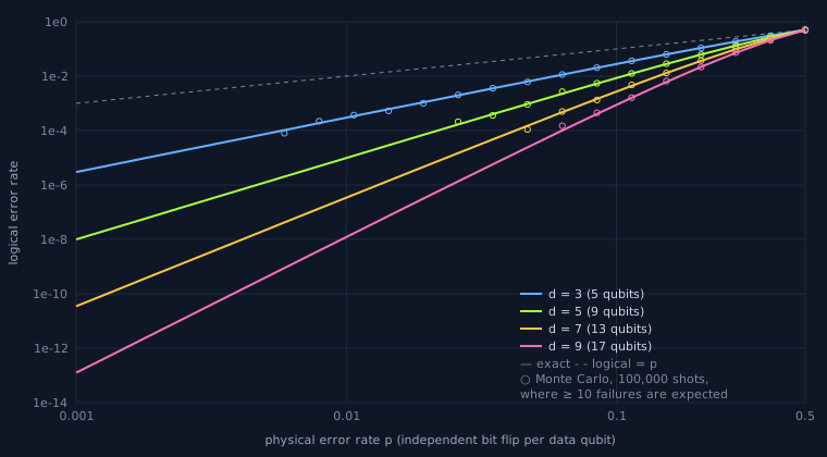
Noise model. A bit-flip repetition code of distance d keeps logical |0⟩ on d data qubits, with d − 1 ancillas measuring neighbouring parities. Each data qubit flips (X) independently with probability p; gates and syndrome measurements are perfect; a minimum-weight decoder picks the correction.
Exact, and what it checks. There are only 2ᵈ error patterns. Each is run once through the syndrome circuit on our NumPy state-vector engine (the TechUPGRADE engine's quantum module; tools/repetition_sweep.py calls it, and computes the closed form beside it), and the logical error rate is the sum of the failing patterns' probabilities. For this noise model a closed form exists — the binomial tail Σk>d/2 C(d,k) pᵏ(1−p)ᵈ⁻ᵏ — and the two agree to 6 × 10⁻¹⁶. That agreement is close to guaranteed: bit flips on |0…0⟩ keep the state a single basis state, so it tests the circuit's logic, not superposition or phase. The test of those is the cross-check against Qiskit below. A Monte Carlo experiment with 100,000 shots per point (seed 20261029) is drawn beside it.
What it does not show. Circuit-level noise — errors in the gates and in the syndrome measurement itself — has no simple formula, and is where real study begins. That, and codes beyond the roughly 20 qubits a state vector allows, need a stabilizer simulator; both are on our list (see Where we are).
Data (CSV, 88 rows) · Chart (SVG) · computed on the simulation engine we built for TechUPGRADE, 29 October 2026; the generator is tools/repetition_sweep.py in the repository
How to reproduce the results: a step-by-step page: the sweep recomputed with public code (Python and NumPy), every row compared with the published data, in seconds; the Monte Carlo counts come out equal.
The surface code under circuit noise,
checked against Stim.
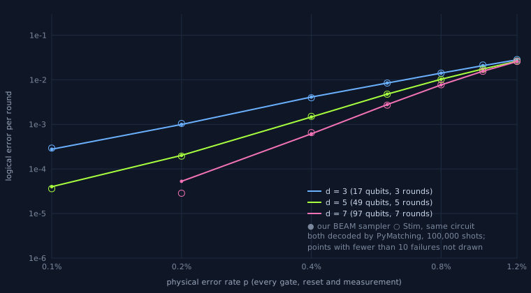
The simulator. QxStab, a stabilizer simulator written in Elixir: a tableau (Aaronson–Gottesman) runs each circuit once without noise for a reference, then a Pauli-frame sampler runs the shots, bit-packed — 1,024 shots in one integer per qubit — in parallel batches, one BEAM process each. It is the method Stim uses, written for the BEAM.
The experiment. Rotated surface codes of distance 3, 5 and 7 (17, 49 and 97 qubits) keep a logical |0⟩ for d rounds of stabilizer measurements. Noise at rate p everywhere: depolarizing after every gate (one- and two-qubit), bit flips after resets and before measurements, depolarizing on the data at each round.
Validation, and what it covers. Each circuit is written out in Stim's format: Stim accepts every detector as deterministic and finds the code distance d for each (our first CNOT order gave only (d+1)/2, a hook-error mistake Stim caught). The detector error model, and so the decoding, comes from Stim; what is compared is the sampling alone. Sampled by Stim and by us, both decoded by PyMatching: the logical error rates agree. Stricter, with exact binomial tests (our count against Stim's, given their sum): every detector's firing rate at all 21 points (3,360 tests, 0.30 % below p = 0.0027 against 0.27 % expected); every detector together with the logical observable, the correlation that sets the logical error rate (3,360 tests, 0.36 %); every pair of detectors for d = 5 at p = 0.6 % (7,140 tests, 0.18 %); and the decoded logical error rates themselves (21 tests, the smallest p-value 0.70 after Bonferroni correction). The detectors are not independent, so these shares are a guide, not a calibrated test. The tests have power: Stim at p = 0.65 % against Stim at 0.6 % is flagged on 97 % of detectors (numbers, tools/stim_exact.py).
What it shows. The curves cross between p = 0.6 % and 0.8 % — three distances and seven error rates bracket the crossing, they do not estimate it (that would need finer steps near it and a finite-size fit). The bracket is in line with published values for this noise model, roughly 0.5 to 1 %: below it, a larger code protects better. The decoder is PyMatching's, not ours.
Data (CSV, 21 points, 100,000 shots each) · Chart (SVG) · tools/beam_runs.exs, tools/stab_study.py · stim 1.16.0, pymatching 2.4.0
How to reproduce the results: a step-by-step page: the BEAM and the tools in two pinned images, about 7 minutes; every count must equal the published one.
Measured against Qiskit Aer and Stim,
including where we lose.
| qubits | gates | QxSim (BEAM) | our NumPy engine | Qiskit Aer |
|---|---|---|---|---|
| 8 | 120 | 1.1 (1.0) | 0.6 (0.6) | 3.5 (3.2) |
| 10 | 190 | 4.5 (4.4) | 1.2 (1.2) | 4.7 (4.6) |
| 12 | 276 | 28.1 (28.0) | 2.7 (2.6) | 7.9 (7.5) |
| 14 | 378 | 199 (176) | 8.4 (8.3) | 8.6 (8.3) |
| 16 | 496 | 1,304 (1,137) | 36.3 (36.0) | 78.7* (42.1) |
| 17 | 561 | 2,994 (2,924) | 81.1 (80.8) | 29.1 (27.2) |
| 18 | 630 | 6,394 (5,528) | 196 (192) | 90.5 (69.6) |
| 19 | 703 | 20,542 (13,645) | 585 (575) | 210 (138) |
| 20 | 780 | out of memory | 1,933 (1,867) | 208 (203) |
The circuit: n layers of Rx on every qubit and CNOTs on neighbours, then 1,024 shots. Timed: building the state and sampling, after one warm-up run; Qiskit's transpilation is not timed. QxSim keeps the state as an Erlang tuple of boxed complex numbers, in one process, rebuilt for every gate: fine for teaching circuits, and about 100 times slower than Aer at 19 qubits; at 20 it runs out of its 1 GB container. Our NumPy engine runs with OpenBLAS on one thread: with its default of 20 threads, each one-qubit gate (a 2×2 matrix against 2ⁿ⁻¹ columns, through tensordot) spent its time starting threads — 15 ms per gate at 20 qubits against 3.5 ms on one thread — which made an earlier version of this table jump 15× at 20 qubits. Profiled, not guessed; one thread is also like for like with QxSim, a single process. Aer's times vary a lot from run to run, hence the minimum beside the median. * At 16 qubits Aer's median is above its time at 17: the noisiest point of the run (its minimum, 42.1 ms, is in line), shown as measured.
| circuit | qubits | QxStab, 20 schedulers | Stim, 1 core | Stim, 20 processes | QxStab / Stim ×20 |
|---|---|---|---|---|---|
| repetition d9 | 17 | 14.0 | 14.0 | 1.8 | 8× |
| surface d3 | 17 | 8.5 | 3.2 | 1.1 | 8× |
| surface d5 | 49 | 20.4 | 22.6 | 2.8 | 7× |
| surface d7 | 97 | 124 | 99.0 | 6.4 | 19× |
| surface d9 | 161 | 371 | 193 | 13.6 | 27× |
Timed: for QxStab, the reference tableau and the sampling, batches of 1,024 shots in parallel BEAM processes; for Stim, compiling the sampler and sampling — on one core, and split over 20 worker processes (started before timing). Like for like, on 20 cores, Stim is 8 to 30 times faster. Against one Stim core our sampler is between 2.8 times slower and about even. What the BEAM offers is not speed but a simple way to spread shots over cores and machines, with batches that cannot crash one another — and Stim spreads just as easily.
Data (CSV) · where: one machine, 20 Arm (aarch64) cores; QxSim and QxStab in the quanterall_quantum container (1 GB memory limit, 20 schedulers), Python on the host (OpenBLAS on one thread) · stim 1.16.0, pymatching 2.4.0, qiskit-aer 0.18.2 (statevector) · tools/beam_runs.exs, tools/stab_study.py
How to reproduce the results: a step-by-step page: the same pipeline as the noise study, and how to compare timings from another machine with ours.
Everything above reproduces known results.
This is the question we want to answer.
Question. Under concurrent load, does a union-find decoder on the BEAM — every syndrome its own lightweight process, many decoded at once on all cores — keep its tail latency bounded, at a throughput near a compiled decoder's?
Baselines, to separate the algorithm from the language. Union-find in a compiled language (Rust or C++), and in plain Python; and PyMatching 2.4 (minimum-weight matching, C++) — each run under the same load as ours: a worker pool on the same cores, fed from a queue, with 1, 100 and 10,000 syndromes in flight. Same machine, same syndromes (sampled by QxStab and by Stim from the threshold-study circuits, d = 3 to 9, p = 0.1 to 1 %). The decoding graph comes from Stim's detector error model for every decoder, ours included: there our work depends on Stim.
The deadline, and why the BEAM. The BEAM is soft real-time: it will not decode for superconducting hardware, whose rounds take about a microsecond. Trapped-ion and neutral-atom machines run rounds of a millisecond or more, and the software that orchestrates any machine works in milliseconds; we test against a 1 ms deadline at d = 5. The question is whether preemptive per-process scheduling keeps the tail there when the queue grows, where a single-threaded decoder's queue waits pile up.
Hypothesis, and what falsifies it. At d = 5: our 99th-percentile latency stays under 1 ms with 10,000 syndromes in flight, growing no more than 2× from 1 to 10,000; and our throughput per core is within 2× of compiled union-find. Either number missing falsifies it. We expect to lose against PyMatching, which decodes such syndromes in microseconds, and we report by how much — and the logical error rate, since union-find is a little less accurate than matching. A partial result still says something: bounded latency at a lower throughput would describe what the BEAM is for.
Protocol. One warm-up pass; 10 repeated runs per point, medians with 95 % intervals by bootstrap; garbage collection left on and reported (BEAM processes collect their own heaps; we record the time spent); scripts, raw timings and syndromes published with the results.
QxDecode (lib/qx_decode.ex): union-find after Delfosse and Nickerson, weighted (edge lengths from the error probabilities, in quarter steps of the lightest edge), peeled over a minimum-weight spanning tree of each cluster. Its first version peeled over a breadth-first tree and failed a simple pattern — two detectors next to each other and the boundary — ten times too often at low noise; comparing with PyMatching shot by shot found it. On the same 100,000 syndromes per point, both on Stim's detector error model:
| d | p | ours | PyMatching | ratio | µs/syndrome, ours, 1 process | µs, PyMatching, 1 core | ours, 20 cores, /s | PyMatching, 1 core, /s |
|---|---|---|---|---|---|---|---|---|
| 3 | 0.1 % | 0.095 % | 0.083 % | 1.145× | 1.6 | 0.04 | 7,001k | 24,748k |
| 3 | 0.4 % | 1.30 % | 1.23 % | 1.057× | 4.5 | 0.11 | 3,800k | 9,407k |
| 3 | 0.6 % | 3.46 % | 2.52 % | 1.372× | 3.1 | 0.16 | 2,637k | 6,415k |
| 3 | 0.8 % | 4.85 % | 4.18 % | 1.161× | 4.3 | 0.21 | 2,004k | 4,716k |
| 5 | 0.1 % | 0.022 % | 0.020 % | 1.1× | 5.0 | 0.33 | 1,779k | 3,076k |
| 5 | 0.4 % | 0.830 % | 0.731 % | 1.135× | 21.5 | 1.01 | 537k | 994k |
| 5 | 0.6 % | 2.83 % | 2.36 % | 1.198× | 34.5 | 1.65 | 367k | 607k |
| 5 | 0.8 % | 6.08 % | 5.04 % | 1.205× | 47.9 | 2.36 | 244k | 424k |
| 7 | 0.1 % | 0.001 % | 0.002 % | 0.5× | 17.2 | 1.23 | 625k | 815k |
| 7 | 0.4 % | 0.528 % | 0.429 % | 1.231× | 83.0 | 4.08 | 152k | 245k |
| 7 | 0.6 % | 2.36 % | 1.93 % | 1.218× | 134.1 | 6.51 | 88k | 154k |
| 7 | 0.8 % | 6.48 % | 5.25 % | 1.234× | 440.2 | 8.82 | 61k | 113k |
What this says. Accuracy: our logical error rate is 1.06 to 1.37 times PyMatching's where both have enough failures to tell (every point except d = 7 at 0.1 %, where the two decoders failed once and twice in 100,000 shots) — union-find's usual distance from matching; McNemar's exact test on the shots where they disagree finds the difference real at most points. Speed: per syndrome on one core we are 14 to 50 times slower than PyMatching; on all 20 cores our throughput is 0.3 to 0.8 of one PyMatching core (about half at d = 5). That is the throughput half of the hypothesis already answered for PyMatching (we lose, as expected); the comparison against compiled union-find and the latency under load follow below (data, tools/dem_graph.py, tools/decode_runs.exs, tools/decoder_compare.py).
First, our design had a flaw. With a fixed number of syndromes in flight, Little's law makes the mean latency that number divided by the throughput: 10,000 in flight at 1 ms needs 10 million syndromes a second from any decoder. That measures throughput, not scheduling. We kept the closed-loop runs, and added the usual test: syndromes arriving at random (Poisson) at 50, 80 and 95 % of what each decoder sustains through its own harness, and the latency from arrival to answer.
The setup. The same 8 fast cores (of a 20-core Arm machine that also runs other services) for every decoder; the same graph and syndromes at p = 0.4 %. QxDecode on 8 BEAM schedulers, one process per syndrome, released by a dispatcher that spins on the clock; union-find in C++ (tools/load/uf.cpp, the same algorithm: identical predictions on 99.94–100 % of shots), a spinning dispatcher and 7 worker threads; PyMatching and union-find in Python, a dispatcher and 7 worker processes. Each harness also ran with a decoder that does nothing, to show its own cost. 10 seeds at d = 5, 3 at d = 3 and 7; medians.
| d | decoder | decode only, /s | through harness, /s | p99 at 50 % | at 80 % | at 95 % | over 1 ms at 50 % | no-op p99 at 50 % |
|---|---|---|---|---|---|---|---|---|
| 3 | QxDecode, BEAM | 2,588k | 505k | 4.29 ms | 6.23 ms | 7.74 ms | 2.4 % | 2.41 ms |
| 3 | union-find, C++ | 15,900k | 4,622k | 310 µs | 2 µs | 2 µs | 0.0 % | 1 µs |
| 5 | QxDecode, BEAM | 331k | 184k | 1.24 ms | 13.57 ms | 8.53 ms | 1.2 % | 45 µs |
| 5 | union-find, C++ | 3,940k | 3,671k | 1.58 ms | 1.49 ms | 1.98 ms | 2.8 % | 1 µs |
| 7 | QxDecode, BEAM | 92k | 59k | 751 µs | 3.07 ms | 25.40 ms | 0.6 % | 36 µs |
| 7 | union-find, C++ | 1,358k | 1,329k | 14 µs | 20 µs | 108 µs | 0.0 % | 1 µs |
Against the hypothesis, at d = 5. Throughput within 2× of compiled union-find: no — 12 times less decoding alone, 20 times less through the harness. 99th percentile under 1 ms: at half load 1.24 ms (95 % interval 894 µs–1.73 ms), at 80 % 13.57 ms, at 95 % 8.53 ms. Growth bounded: no. The hypothesis is falsified.
What it does show. A process per syndrome costs the BEAM more than the decoding: its harness alone, with no decoding, has a 99th percentile of 2.41 ms at half load for d = 3 — spawning and messaging at a few hundred thousand a second is the bottleneck, not the scheduler's fairness. C++'s tails are bimodal across seeds — microseconds in some runs, milliseconds in others — which fits interference from the machine's other work on shared cores; a clean tail measurement needs a machine to itself. Python's harness costs more than any deadline here (its no-op p99 is tens of milliseconds), so for PyMatching and Python union-find only throughput is meaningful: about 124k and 93k syndromes a second through it at d = 5.
Next. Decode many syndromes per process (batches) rather than one each, to separate the BEAM's scheduling from its spawning cost; a dedicated machine for the tails; then the question again. Data: summary, every run; tools/load/.
The science of
superposition
A register of n qubits is described by 2n complex amplitudes. A measurement returns one outcome, with probability given by its amplitude squared; the amplitudes themselves are never read out. So n qubits do not compute 2n results and hand them all back: each run yields one n-bit outcome. Speedups come from interference: an algorithm arranges the amplitudes so that wrong answers cancel and right ones reinforce before that one measurement.
|ψ⟩ = α|0⟩ + β|1⟩, |α|² + |β|² = 1